The Boltzmann Distribution

2022 Mar 15

This is the first post on this website. Welcome! Since the first post is a bit of special one, I'll have to make it about something important. The Boltzmann distribution is very important, so let's go with that.

The Boltzmann distribution is a probability distribution that shows up in physics. We have some system, like a lump of iron or some gas in a box, which could be in many different states. We have a good idea of the overall energy of the system, but maybe we don't know much else about it. Actually, according to quantum mechanics, if we knew the energy exactly the system would never evolve. So let's say that we only know the expected value of the energy, U. Question: What is the probability distribution over states of the system?

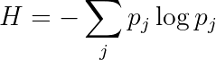
The probability distribution over states will be one with maximum entropy, of course. That's how it always is in these kinds of physics questions. Systems like to exchange information with their environment, picking up thermal noise until they're packed to the brim with it. Just so we can talk about the probability distribution over states, we'll assign a number j to each state. And we'll write the probability of that state as pⱼ. Then the entropy can be written as:

$H = -\sum_{j} p_j \log p_j$

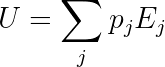
This is what we want to maximize. There is also a constraint on the distribution, namely that the expected value of energy must be U. We'll write the energy of state j as Eⱼ.

$U = \sum_{j} p_j E_j$

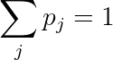
Actually, there's one more invisible constraint: the probabilities must sum to 1:

$\sum_{j} p_j = 1$

Now we can solve this system given the constraints using the method of Lagrange multipliers. Just as a reminder of how this goes, we define multipliers for each constraint: β for the expected energy constraint, and λ for the normalization constraint. This gives us the following equation to solve:

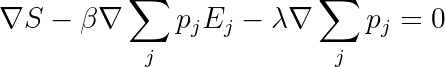
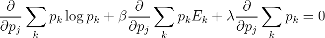
$\nabla S - \beta \nabla\sum_{j} p_j E_j - \lambda \nabla\sum_{j} p_j = 0$

Of course, the solution must still be subject to the constraints. We can break the gradient into components to obtain the following formula (true for all j):

$\frac{\partial}{\partial p_j} \sum_k p_k \log p_k + \beta \frac{\partial}{\partial p_j} \sum_k p_k E_k + \lambda \frac{\partial}{\partial p_j} \sum_k p_k = 0$

$\log p_j + 1 + \beta E_j + \lambda = 0$

$p_j = \exp(-(\beta E_j + \lambda+1))$

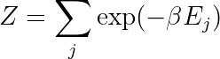
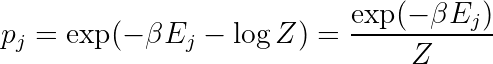
Normalization is more fundamental, so we'll start by enforcing that. We define a new quantity Z as follows. The λ+1 just gives a multiplicative factor, and we're trying to solve for λ so we leave that out of the definition:

$Z = \sum_j \exp(-\beta E_j)$

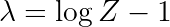
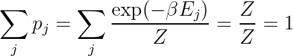
Now we can choose λ so that the probabilities sum to one:

$\lambda = \log Z - 1$

$p_j = \exp(-\beta E_j - \log Z) = \frac{\exp(-\beta E_j)}{Z}$

$\sum_j p_j = \sum_j \frac{\exp(-\beta E_j)}{Z} = \frac{Z}{Z} = 1$

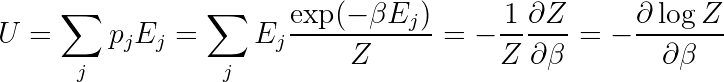
Now we just need to enforce the expected energy constraint.

$U = \sum_j p_j E_j = \sum_j E_j \frac{\exp(-\beta E_j)}{Z}$

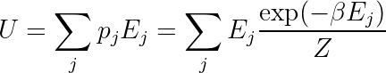
How to solve this depends on the exact nature of the system. The equation is a sum of exponentials, so it could be quite difficult to get an analytic solution in general. But there is a nice expression in terms of Z:

$U = \sum_j p_j E_j = \sum_j E_j \frac{\exp(-\beta E_j)}{Z} = -\frac{1}{Z} \frac{\partial Z}{\partial \beta} = -\frac{\partial \log Z}{\partial \beta}$